Tychos MathJs Language Reference

The following reference guide identifies the language syntax, built in variables, functions, and classes that are used to code your simulations in Tychos. Tychos uses the MathNotepad language. We have included documentation here for some of the helpful functions defined in the MathNotepad language. This is not a complete list of all functions available in MathNotepad, just ones that might be commonly used in Tychos for building scenarios as well as defining goals for those scenarios.

Comments

Comments are statements that you can insert in your code that do not get interpreted and executed by Tychos. To create a comment, you simply indicate a comment by using a hashtag:

# This is a comment.

Variables

To define a variable in Tychos all you need to do is identify a name for the variable. You then type an = sign to assign a value to the variable. The following demonstrates various variable declarations

# Assigns a variable called x the value of 10
x = 10
# Assign a new variable y the value of the x
y = x
# Assign x the value of itself plus 1
x = x + 1

Built-in Scenario Variables

There are a few variables that are built into Tychos. These variables are:

  • t — How many seconds has passed since this Scenario was started?

  • dt — Time between frames as seconds, e.g. 0.1 is 1/10th of a second.

  • frame_count — How many frames have passed? e.g. 1, 2, 3...

  • X, Y , Z— These are shortcuts for indexing the first two elements of 3-D matrices, e.g. my_particle.pos[X]

Common Math Operators and Functions

These are some common mathematical operators and functions for performing various calculations.

Mathematical Operators

Tychos uses the following operators to perform basic math calculations:

  • + — Addition

  • - — Subtraction

  • * - Multiplication

  • / - Division

  • ^ - Exponent

  • % - Modulo

Basic Math Functions

You can also use the following basic math functions:

pow(base, power)

The pow(base, power) function takes two arguments, raising the base by the power.

# returns number 8
pow(2,3)

sqrt(positive_number)

The sqrt(positive_number) function takes a single non negative number and returns the real square root of the number.

# returns number 2
sqrt(4)

abs(number)

The abs(number) function returns the absolute value of a number.

# returns number 2
abs(-2)

Trigonometric Functions

The following functions all use radians as the angle measurement. You can use pi to represent PI.

sin(angle)

The sin(angle) function is used to evaluate the trigonometric sine value for a given input angle. The input angle must be provided in radians.

# returns number 1
sin(PI/2)

cos(angle)

The cos(angle) function is used to evaluate the trigonometric cosine value for a given input angle. The input angle must be provided in radians.

# returns number 1
cos(0)

tan(angle)

The tan(angle) function is used to evaluate the trigonometric tangent value for a given input angle. The input angle must be provided in radians.

# returns number 1
tan(PI/4)

asin(value)

The asin(value) function is used to evaluate the trigonometric arcsine value (inverse sine) for a given input. The output angle is given in radians.

# returns number 1.57
asin(1)

acos(value)

The acos(value) function is used to evaluate the trigonometric arccosine value (inverse cosine) for a given input. The output angle is given in radians.

# returns number 0
acos(1)

atan2(X, Y)

The atan2(value) function is used to evaluate the trigonometric arctangent value (inverse tangent) for a given X and Y input. The output angle is given in radians.

# returns number -0.785
atan2(-1, 1)
# returns 2.36
atan2(1, -1)

deg_to_rad(angle)

See below.

radians(angle)

The deg_to_rad(angle) function is not part of the MathNotepad language but is provided as a helper function to make the conversion from degree angles to radians easier. The input is an angle measurement in degrees and the output is the angle measurement in radians.

# returns number .785
deg_to_rad(45)

rad_to_deg(angle)

See below.

degrees(angle)

The degrees(angle) function is not part of the MathNotepad language but is provided as a helper function to make the conversion from radian angles to degrees easier. The input is an angle measurement in radians and the output is the angle measurement in degrees.

# returns number 180
degrees(PI)

Matrix Functions

The following functions provide operations for matrix calculations.

dot(x, y)

Calculates the dot product of two vectors. The dot product of x = [a1, a2, a3, ..., an] and y = [b1, b2, b3, ..., bn] is defined as:

dot(x, y) = a1 * b1 + a2 * b2 + a3 * b3 + … + an * bn

# Work is the dot product of Force (F) and displacement (r)
F = [2, 2]
r = [3, 3]
# returns 12
Work = dot(F, r)

cross

Calculates the cross product for two vectors in three dimensional space. The cross product of x = [a1, a2, a3]and y = [b1, b2, b3] is defined as:

cross(x, y) = [ a2 * b3 - a3 * b2, a3 * b1 - a1 * b3, a1 * b2 - a2 * b1 ]

If one of the input vectors has a dimension greater than 1, the output vector will be a 1x3 (2-dimensional) matrix.

# Torque is the cross product of Force and moment arm (r)
F = [2, 0, 0]
r = [0, 2, 0]
# returns matrix [0, 0, 4]
cross(F, r)

Other Useful Functions

Some other useful functions...

random(min, max)

Return a random number larger or equal to min and smaller than max using a uniform distribution. If now min or max are given, then it returns a random value from 0 to 1. If just one value is given, then it returns a random number between 0 and the input value.

# returns a random number between 0 and 1
random()
# returns a random number between 0 and 100
random(100)
# returns a random number between 30 and 40
random(30, 40)
# returns a 2x3 matrix with random numbers between 0 and 1
random([2, 3])

string(object)

Create a string or convert any object into a string. Elements of Arrays and Matrices are processed element wise.

format(value, precision)

Formats a value into a string. You have several options for how this value will be formatted:

# returns '0.333'
format(1/3, 3)
# returns '21000'
format(21385, 2)
# returns '1200000000'
format(12e8, {notation: 'fixed'})
# returns '2.3000'
format(2.3,  {notation: 'fixed', precision: 4})                

concat(A, B...dim)

Concatenate two or more matrices. This function can also be used to concatenate strings together.

dim: number is a zero-based dimension over which to concatenate the matrices. By default the last dimension of the matrices.

A = [1, 2]
B = [3, 4]
concat(A, B)                  
# returns [1, 2, 3, 4]
math.concat(A, B, 0)           
# returns [[1, 2], [3, 4]]
math.concat('hello', ' ', 'world') 
# returns 'hello world'

drawArrow (deprecated)

This function has been deprecated and you should instead use the class Arrow to represent arrows in your simulations. See below for more details.

The drawArrow function draws an arrow and is commonly used to illustrate vectors for a particle. drawArrow should be called in the Calculations editor because it only draws the arrow for the current frame. If you call drawArrow() in the Initial State editor, you will not see anything.

drawArrow(pos=[0,0], size=[1,0], color="black", components=false, thickness=1) -> returns and draws an Arrow object

  • pos — coordinates for the starting point of the arrow as an [X,Y] matrix.

  • size — the vector to illustrate, e.g. [10, 0] will draw an arrow 10 units to the right.

  • color — Optional HTML color value for your arrow, e.g. "red" or "#ff0000".

  • components — Optional flag that determines if vector components are drawn, a value of true displays the components.

  • thickness — Optional stroke value that determines the visual thickness of the arrow.

drawLine (deprecated)

This function has been deprecated and you should instead use the class Line to represent lines in your simulations. See below for more details.

The drawLine function draws a line and is commonly used to illustrate some connecting member like a string or cable, but could really represent anything you like. drawLine should be called in the Calculations editor because it only draws the line for the current frame. If you call drawLine in the Initial State editor, you will not see anything.

drawLine(pos=[0,0], pos2=[10,0], color="black", thickess=1) -> returns and draws an Line object

  • pos — coordinates for the starting point of the line as an [X,Y] matrix.

  • pos2 — the coordinates of the end point of the line as an [X,Y] matrix.

  • color — Optional HTML color value for the line, e.g. "red" or "#ff0000".

  • thickness — Optional stroke value that determines the visual thickness of the line.

Example — The illustration above was drawn using this command:

# Calculations editor
drawLine([0, 0], [20, 20], "purple", 2)  # a line
drawLine([0, 0], [10, 20], "green", 10)  # another line

unit_vector

This function returns a unit vector representation of the given input vector. Its magnitude is 1 and the direction matches the direction of the input vector. This can be useful if you need just the direction of a vector, but not its magnitude.

unit_vector(vec) -> returns a vector of length 1, and in same direction as vec.

  • vec - any two dimensional vector as a [X, Y] matrix.

Example:

u = unit_vector([3, 4])  # returns [0.6, 0.8]
magnitude(u)             # returns 1

magnitude

This function returns the scaler magnitude of any given vector. This is helpful when you want to know the length of a vector, for example, if you want the magnitude of a vector, but not its direction.

magnitude(vec) -> returns the scaler magnitude of the vector vec.

  • vec - any two dimensional vector as a [X, Y] matrix.

Example:

magnitude([3, 4])             # returns 5

direction

This function returns a scalar angle measurement. This is helpful when you want to know the direction of a vector, like the direction of a velocity vector, or the direction of a force vector. The default return angle is given in radians, but can also be expressed in degrees.

direction(vec, units="rad") -> returns the scaler angle measurement of the vector vec heading in radian form or in degree form.

  • vec - any two dimensional vector as a [X, Y] matrix.

  • units - optional deg for degree measurement or the default of rad for radians.

Example:

direction([4, 4])             # returns .785
direction([4, 4], "deg")        # returns 45

polar

This function returns a two-dimensional matrix representing the cartesian components of a polar coordinate corresponding to the magnitude of the radius and the radial angle.

polar(radius, angle, units="rad") -> returns a two dimensional vector as a [X, Y] matrix.

  • radius - scalar quantity representing the scalar distance of the radius of the

  • angle - scalar quantity representing the angle measurement of the polar coordinate.

  • units - optional deg for degree measurement or the default of rad for radians.

Example:

polar(10, 45, "deg")         # returns [7.07, 7.07]
polar(10, PI/4)            # returns [7.07, 7.07]

stop

This function actually evaluates a boolean test and then stops the simulation once the boolean test succeeds. This can be useful if you want the simulation to stop when some condition has been met within your simulation.

stop(test) -> returns a either false or true. If true is returned, the simulation stops.

  • test - a boolean statement that can be evaluated to true or false.

Example:

stop(t > 10)             # simulation stops at 10 seconds
stop(buggy.pos[X] == 100) # simulation stops when X position of particle equals 100

Collision Functions

The following functions are meant to help users model collisions more easily. These functions could be used for other purposes rather than modeling collisions as Tychos is not a physics engine. These functions could be thought of as "overlap" functions. They return information about the overlap of objects.

hasCollided

This function returns a boolean true/false value when two objects are given as the source and target. It returns false if the two objects are not determined to be overlapping.

hasCollided(source, target) -> returns a boolean true or false.

  • source - Circle or Rectangle object

  • target - Circle or Rectangle object

Example:

# Initial State
p1 = Circle({pos:[15, 0], radius:10, color:rgba(0, 200, 200, .6)})
b1 = Rectangle({pos:[0, 0], size:[15, 15], color:rgba(200, 0, 200, .6)})
b1.rotate(radians(45))
p3 = Circle({pos:[-15, 0], radius:10, color:rgba(0, 0, 200, .6)})
# Calculations
hasCollided(p1, b1)            # returns true
hasCollided(b1, p3)            # returns true
hasCollided(p1, p3)            # returns false

getIntersect

This function returns a two dimensional matrix representing the minimum translation vector (MTV) that would be needed to separate two objects when they overlap. This can be used to simulate collision forces or to move objects apart based on the magnitude and direction of the MTV.

getIntersect(source, target) -> returns a two dimensional matrix.

  • source - Circle or Rectangle object

  • target - Circle or Rectangle object

Example:

# Initial State
p1 = Circle({pos:[0, 0], radius:10, color:rgba(200, 200, 200, .6)})
p2 = Circle({pos:[12, 10], radius:10, color:rgba(0, 200, 0, .6)})
b1 = Rectangle({pos:[-12, 0], size:[15, 15], color:rgba(200, 0, 0, .6)})
mtv1 = Arrow({pos:[p1.pos], color:"green"})
mtv2 = Arrow({pos:[p1.pos], color:"red"})
# Calculations
mtv1.size = getIntersect(p1, p2)
mtv2.size = getIntersect(p1, b1)

Comparison Functions

The following functions are used to compare two values as being equal or unequal as well as testing if one value is larger or smaller than another. These are very helpful when writing goals for students.

equal(a, b) or a == b

The function tests if two values (x and y) are equal. It returns a boolean value of true or false.

2 + 2 == 3             # returns false
2 + 2 == 4             # returns true
t == 10                # returns true if t is 10, or false if it is not.
equal(2 + 2, 4)        # same as 2 + 2 == 4

deepEqual(a, b)

This function is similar to equal, but it tests element wise whether two matrices are equal. It returns a boolean value of true or false. The code below demonstrates the difference between equal and deepEqual:

p1 = Particle([10, 10])
p2 = Particle([10, 0])
deepEqual(p1.pos, p2.pos)   # returns false
equal(p1.pos, p2.pos)       # returns [true, false]

larger(a, b) or a > b

The function tests if one value (a) is larger than another (b). It returns a boolean value of true or false.

2 > 3               # returns false
3 > 2               # returns true
2 > 2               # returns false
larger(2, 2)        # same as 2 > 2

smaller(a, b) or a < b

The function tests if one value (a) is smaller than another (b). It returns a boolean value of true or false.

2 < 3                # returns true
3 < 2                # returns false
2 < 2                # returns false
smaller(2, 2)        # returns false

unequal(a, b) or a != b

The function tests if two values (a and b) are unequal. It returns a boolean value of true or false.

2 + 2 != 3              # returns true
unequal(2 + 2, 3)       # true -- same as 2 + 2 != 3
2 + 2 != 4              # returns false
t != 10                 # returns false if t is 10, or true if it is not.

Comparison operators return true or false but these also evaluate to 1 (true) or 0 (false). This can allow you to conditionally assign a value to a variable depending on the evaluation of the comparison. See the code below as an example:

# If t is larger than 10, then the value of F is [10, 10], otherwise it is 0.
F = (t > 10) * [10, 10]

if(test, true_result, false_result)

The if() function returns true_result or false_result depending on test.

if(true, 3, 44)                 # returns 3
if(false, 3, 44)                # returns 44
if(1 > 2, 3, 44)                # test is false; therefore returns 44
a = 1
b = 1
if(a == b, "YAY", "darn")       # test is true; therefore returns "YAY"

Logical Operators

The following operators are used to execute logical AND and OR comparisons for the use of evaluating logical statements.

and

This is used for performing a logical AND conjunction. For example, "A and B" is true only if A is true and B is true. "A and B" is false if either A or B is false.

A = true
B = true
A and B         # returns true
B = false
A and B         # returns false

You can use the and operator to test if two comparisons are both true:

x = 2
(x < 3) and (x == 2)  # returns true
(x < 3) and (x != 2)  # returns false

or

This is used for performing a logical OR conjunction. For example, "A or B" is true if A or B is true. "A or B" is false only if A and B are both false.

A = true
B = false
A or B # returns true
A = false
A or B # returns false

You can use the or operator to test if one of two comparisons are true:

x = 2
smaller(x, 3) or equal(x, 3)    # one is true, so returns true
(x < 1) or (x == 3)             # both are false, so returns false

Built-in Classes

Tychos has only a few classes that are used to create the basic simulated objects in the Tychos universe as well as a few tools for analyzing those objects in the simulated world. The graphical objects in Tychos that can be used are the Cirlcle, the Rectangle, the Arrow, the Line, the Label, and the Spring The tools that can be used for analyzing the behavior of your simulations are the Graph, the Gauge and the Meter. There are also user input objects that can be added to your simulations to make them more interactive: the Toggle, the Slider, the Input, and the Menu controls.

Circle

A Circle is drawn as a colored circle in the World View. A Circle has a position, a radius, a color, an opacity, a flag for setting its visibility state, and a flag for determining if a motion map should be attached.

Below is the constructor for the Circle class that shows its default values:

Circle(
  {pos:[0,0], 
   radius:10, 
   color:default_color, 
   image: "",   
   opacity: 1, 
   visible: true, 
   motion_map: false,
   label: {text: "", color: default_color}
  }
) 
  • pos — The initial position of your Circle in [X,Y] coordinates.

  • radius — The radius of the circle that is drawn in the World View to represent this particle.

  • color — The circle will be drawn in this color. Use HTML colors e.g. "#ff3300", "blue".

  • image — A URL that identifies a JPEG, GIF, SVG or PNG image.

  • opacity — The circle will be drawn with an opacity between 1 and 0, representing 100% opaque to 100% transparent.

  • visible — The circle can be hidden from view by setting this flag to false.

  • motion_map — This flag tells Tychos to attach a series of strobe images called a motion map.

  • label - You can attach a label to the Circle object by indicating a the text and color of the label.

These attributes may also be modified on the Circle after it is created. In particular, one will usually change the pos attribute of a Circle in the Calculations editor to show movement. e.g.

# Initial State editor
c = Circle()
c_big = Circle({pos:[50, 0], radisu:25})
c_big.color = "red"
c_green = Circle({pos:[100, 0], color: "green", opacity: .5})
# Calculations editor
c.pos = c.pos + [1, 0.25]

Circle.rotate()

Circle objects can be rotated.

Circle.rotate(angle=0, axis=[0, 0]) — Rotates the Circle object by a given angle value in radian units. You can also provide an optional matrix that identifies the axis of rotation. This method should only be called from the Calculations code editor.

Circle.image

Circle objects can also be represented with an image by setting the image attribute of the object. The text must be a URI link to a graphic file that can be a PNG, SVG, GIF, or JPEG image.

rocket = Circle({pos:[0, 0], radius:10})
rocket.image = "https://upload.wikimedia.org/wikipedia/commons/3/3d/Spacecraft.png"

The above image also demonstrates the use of the direction function as well as the rotate method:

rocket.rotate(direction(rocket.v))

Circle.label

Circle objects can also be given a text label. This is similar to the Label object.

c.label = {text:"Hello", color:"green"} — This adds a text label to the Circle object that scales to fit inside the circle.

Rectangle

A Rectangle is very similar to a Circle but it is represented as a colored rectangle in the World View. A Rectangle has position, width, height, color, opacity, visibility, a motion map flag, as well as a label. Just as with the Circle, Tychos only uses the width and height attributes for display. You can define how these attributes change given the rules of the simulation that you define.

Below is the constructor for the Rectangle class that shows its default values:

Rectangle(
  {pos:[0,0], 
   size:[10,10], 
   color:default_color,
   image: "", 
   opacity: 1, 
   visible: true, 
   motion_map: false,
   label: {text: "", color: default_color}
  }
)
  • pos — The initial position of your Rectangle in [X,Y] coordinates.

  • size — The width and height of the Rectangle that is drawn in the World View to represent this particle.

  • color — The Rectangle will be drawn in this color. Use HTML colors e.g. "#ff3300", "blue".

  • image — A URL that identifies a JPEG, GIF, SVG or PNG image.

  • opacity — The Rectangle will be drawn with an opacity between 1 and 0, representing 100% opaque to 100% transparent.

  • visible — The Rectangle can be hidden from view by setting this flag to false.

  • motion_map — This flag tells Tychos to attach a series of strobe images called a motion map.

  • label - You can attach a label to the Rectangle object by indicating a the text and color of the label.

These attributes may also be modified on the Rectangle object after it is created. In particular, one will usually change the pos attribute in the Calculations editor to show movement. e.g.

# Initial State editor
r1 = Rectangle({pos:[0, 0], size:[10, 10], color:"green"})
r2 = Rectangle({pos:[20, 0], size:[10, 20], color:"blue"})
r3 = Rectangle({pos:[40, 0], size:[20, 10], color:"orange"})
# Calculations editor
r1.pos = r1.pos + [1, 0.25]

Rectangle.rotate

You can also rotate a Rectangle object in order to simulate rotational behavior.

Rectangle.rotate(angle=0, axis=[0, 0]) — Rotates the Rectangle object by a given angle value in radian units. You can also provide an optional matrix that identifies the center of rotation. This method should only be called from the Calculations code editor.

Example:

# Calculations editor
r1.rotate(-PI/4)
r2.rotate(radians(90))
r3.rotate(radians(45))

Rectangle.image

Just as with Circle objects, Rectangle objects can also be represented with an image by setting the image attribute of the object.

r.image = "https://some.image.url.jpg"

Rectangle.label

Rectangle objects can also be given a text label. This is similar to the Label object.

r.label = {text:"Hello", color:"green"}

This adds a text label to the Rectangle object.

Arrow

The Arrow class represents a graphical arrow and is commonly used to illustrate vectors, but can be used for representing anything in your simulations.

Below is the constructor for the Arrow class that shows its default values:

Arrow(
  {
    pos:[0,0], 
    size:[1,0], 
    color:default_color,
    componets: false,
    stroke: 1, 
    opacity: 1, 
    visible: true, 
    motion_map: false
 }
)
  • pos — coordinates for the starting point of the Arrow as an [X,Y] matrix.

  • size — the vector to illustrate, e.g. [10, 0] will draw an Arrow 10 units to the right.

  • color — HTML color value for your Arrow, e.g. "red" or "#ff0000".

  • components — A flag that determines if X and Y components are drawn, a value of true displays the components.

  • stroke — Stroke value that determines the visual thickness of the Arrow.

  • opacity — The Arrow will be drawn with an opacity between 1 and 0, representing 100% opaque to 100% transparent.

  • visible — The Arrow can be hidden from view by setting this flag to false.

  • motion_map — This flag tells Tychos to attach a series of strobe images called a motion map.

Arrow without components
Arrow with components

Example — The illustrations above were drawn using these commands:

# Initial State editor
c = Circle({pos:[0,0], color:"green"})
a = Arrow({pos: c.pos, size: [20, 20], color:"purple"})
a.components = true

Line

The Line class draws a line and is commonly used to illustrate some connecting member like a string or cable, but could really represent anything you like.

Below is the constructor for the Line class that shows its default values:

Line(
  {
   pos:[0,0], 
   pos2:[1,0], 
   color:default_color,
   stroke: 1, 
   opacity: 1, 
   visible: true, 
   motion_map: false
  }
)
  • pos — coordinates for the starting point of the Line as an [X,Y] matrix.

  • pos2 — coordinates of the termination point of the Line as an [X,Y] matrix

  • color — HTML color value for your Line, e.g. "red" or "#ff0000".

  • stroke — Stroke value that determines the visual thickness of the Line. This is measured in pixels.

  • opacity — The Line will be drawn with an opacity between 1 and 0, representing 100% opaque to 100% transparent.

  • visible — The Line can be hidden from view by setting this flag to false.

  • motion_map — This flag tells Tychos to attach a series of strobe images called a motion map.

Example:

myLine = Line({pos:[0, 0], pos2: [20, 20], color: "purple", stroke:2})
anotherLine = Line({pos:[0, 0], pos2: [10, 20], color: "green", stroke:10})

PolyLine

The PolyLine class displays a sequence of straight lines between points, and is commonly used to illustrate a more complex shape or path.

Below is the constructor for the Line class that shows its default values:

PolyLine(
  {
   pos:[0,0], 
   color:default_color,
   stroke: 1, 
   opacity: 1, 
   visible: true, 
   style: "none",
   retain: 100
  }
)
  • pos — coordinates for the starting point of the Line as an [X,Y] matrix.

  • color — HTML color value for your Line, e.g. "red" or "#ff0000".

  • stroke — Stroke value that determines the visual thickness of the Line. This is measured in pixels.

  • opacity — The Line will be drawn with an opacity between 1 and 0, representing 100% opaque to 100% transparent.

  • visible — The Line can be hidden from view by setting this flag to false.

Example:

myLine = Line({pos:[0, 0], pos2: [20, 20], color: "purple", stroke:2})
anotherLine = Line({pos:[0, 0], pos2: [10, 20], color: "green", stroke:10})

Spring

A Spring is a visual representation of a common elastic connector that displays a given number of coils that dynamically change shape once the dimensions of the Spring are changed in the Calculations Pane.

Below is the constructor for the Spring class that shows its default values:

Spring(
  {
   pos:[0,0], 
   pos2:[1,0], 
   color:default_color,
   coils: 5,
   width: 10,
   stroke: 1, 
   opacity: 1, 
   visible: true, 
   motion_map: false
  }
)
  • pos — coordinates for the starting point of the Spring as an [X,Y] matrix.

  • pos2 — coordinates of the termination point of the Spring as an [X,Y] matrix

  • color — HTML color value for your Spring, e.g. "red" or "#ff0000".

  • coils — The number "coil" zig-zags.

  • width — The width of the "coil" zig-zags.

  • stroke — Stroke value that determines the visual thickness of the Spring. This is measured in pixels.

  • opacity — The Spring will be drawn with an opacity between 1 and 0, representing 100% opaque to 100% transparent.

  • visible — The Spring can be hidden from view by setting this flag to false.

  • motion_map — This flag tells Tychos to attach a series of strobe images called a motion map.

The code below shows the three different Spring objects above that have different lengths, widths and coil numbers. The Circle objects are shown just for reference.

# Initial State editor
c1 = Circle({pos:[0, 0], radius:2, color:"green"})
spring1 = Spring({pos:[0, 20], pos2:c1.pos, color:"black", coils:20, width:2})
c2 = Circle({pos:[10, 0], radius:2, color:"green"})
spring2 = Spring({pos:[10, 20], pos2:c2.pos, color:"black", coils:10, width:4})
c3 = Circle({pos:[20, 0], radius:2, color:"green"})
spring3 = Spring({pos:[20, 20], pos2:c3.pos, color:"black", coils:20, width:2})

These attributes may also be modified after the Spring is created.

Label

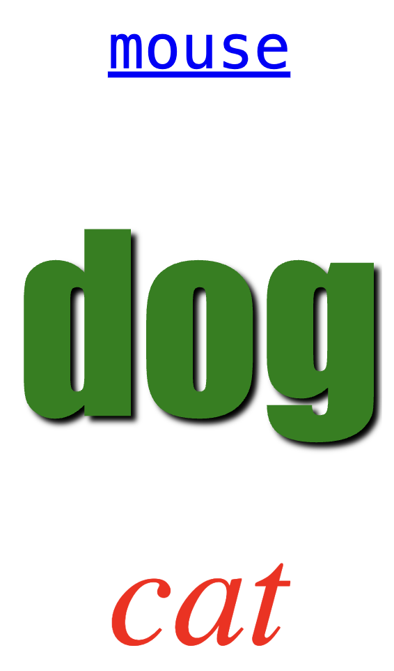
You can add text labels to any scenario using the Label class.


dog = Label({pos:[0,0], size:[20,20], text:"dog", color:"green"})
cat = Label({pos:[0,-15], size:[10,10], text:"cat", color:"red"})
mouse = Label({pos:[0,15], size:[10,10], text:"mouse", color:"blue"})
dog.font="Impact"
cat.font="Times"
mouse.font="monospace"
dog.style = {textShadow:"3px 3px 3px black"}
cat.style = {fontStyle:"oblique"}
mouse.style = {textDecoration:"underline"}

Below is the constructor for the Label class that shows its default values:

Label(
  {
   pos:[0,0], 
   size:[10,10], 
   text: "",
   color:default_color,
   font: "default"
   style: {},
   opacity: 1, 
   visible: true, 
   motion_map: false
  }
)
  • pos — coordinates for the center point of the Label as an [X,Y] matrix.

  • size — The width and height of the Label as an [X,Y] matrix

  • text — The text of the Label as a string.

  • color — HTML color value for your Label, e.g. "red" or "#ff0000".

  • font — CSS font family identifier, e.g. "Times", or "Courier"

  • style — An object with key-value pairs that represent CSS font styling rules.

  • opacity — The Label will be drawn with an opacity between 1 and 0, representing 100% opaque to 100% transparent.

  • visible — The Label can be hidden from view by setting this flag to false.

  • motion_map — This flag tells Tychos to attach a series of strobe images called a motion map.

These attributes may also be modified after the Label object is created.

Label.rotate

Just as with a Rectangle object or a Circle object, you can rotate a Label as shown above:

label3.rotate(PI/4)

World

The world object represents the viewable area of the scenario.

world.set_extents()

You can set the viewable extents of the world in the Settings Pane, or by calling the following method on the world object:

world.set_extents(pos=[0,0], size=[10,10])

The inputs are two vector objects representing the center position of the view of the world, and secondly the size of the viewable world.

Particle (deprecated)

This class has been deprecated. Past scenarios that used this class will NO LONGER work. Please use the Circle class.

Block (deprecated)

This class has been deprecated. Past scenarios that used this class will NO LONGER work, Please use theRectangle class.

Interface Widgets

Tychos also provides several "widgets" for displaying data in different ways as well as adding user interactivity so that your simulations can respond to input.

Graph

A Graph is a 2-dimensional chart of data that you specify in the Calculations editor. Each Graph that is created will appear on the right side of the World View. Your program needs to add points to the graph with the plotcommand.

g1 = Graph({title:"Line Graph", align:"left", width:"50%", height:200})
g1.plot(x=[0,1,2,3], y=[0, 10, 10, 0], color="purple", mode="line", fill=true})
g1.plot(x=[0,1,2,3], y=[0, 2, 4, 9], color="green", mode="line", fill=false})
# Create a graph with a scatter plot.
g2 = Graph({title:"Scatter Graph", align:"right", width:"50%", height:400})
# x_vals and y_vals are lists of numerical points.
g2.plot(x=x_vals, y=y_vals, color="orange", mode="scatter")

Here is the constructor for creating a graph object

Graph(
    {
        title:"Graph", 
        align:"right", 
        y_axis:"Y", 
        x_axis:"X",
        width:500,
        height:350,
        plot_rate:undefined
    }
)
  • title = Optional text that will appear at the top of the graph.

  • align = Optional value of "left" or "right" to align the graph to the corresponding side of the view window.

  • y_axis = Optional text that will appear on the left side of the graph as the vertical axis label.

  • x_axis = Optional text that will appear at the bottom of the graph as the horizontal axis label.

  • width = Optional numeric value in pixels for setting the width, or a text value percentage e.g. "50%" or "90%".

  • height = Optional numeric value in pixels for setting the height, or a text value percentage e.g. "50%" or "90%".

  • plot_rate = Optional numerical value greater than 0 that sets the individual graph's plotting schedule. This over rides the default Graph Strobe Rate value set in the Settings tab.

Plotting Values

To plot values for the graph, the plot method is used. You can either plot points by calling the plot method with the x and y arguments set to single numerical inputs, or to plot more than a single point, you can instead set the x and y arguments to be lists of numerical values.

When plotting, Tychos will plot the points you specify when the simulation plot timer has expired. This is called "strobing" the graph. There is a default plot timer set in the Settings tab called Graph Strobe Rate for the scenario, but this can be over ridden by setting the graph's plot rate.

Note that depending on the simulation step time and the graph plot rate, graph plots may not appear on the graph at the exact time specified by the graph plot rate. For example, if the plot rate is actually faster than the animation step rate, the plotting of the points will not appear to be in sync because the animation is actually running slower than rate at which points should be plotted.

The arguments for the plot method are shown below:

Graph.plot(
    x=0, 
    y=0, 
    color=default_color,
    mode="line",
    fill=False
)
  • x = This is either a single numerical value or a list of numerical values.

  • y = This is either a single numerical value or a list of numerical values.

  • color = Optional "line" or "scatter" that will either display the points as connected with lines, or not. The default is to connect the plotted points with lines.

  • mode = Optional "line" or "scatter" that will either display the points as connected with lines, or not. The default is to connect the plotted points with lines.

  • fill = Optional boolean value for filling in the plotted area.

Clearing Values

To clear values for the graph, the clear method is used. Clearing the plotted values occurs immediately when the method is called, clearing all the plotted values from the graph:

Graph.clear()

BarChart

A BarChart is a chart of data that is displayed as a set of bars representing an array of data values. Each BarChart that is created will appear on the right side of the World View.

# Initial State Pane
bc_energy = BarChart({title:"Energy Bar Chart", min:0, max:500})
bc_energy.setData([150, 250, 200, 500])
bc_energy.setColors(["red", "blue", "green", "black"])
bc_energy.setLabels(["KE", "Ue", "Ug", "TE"])
  • title = Optional text that will appear at the top of the bar_chart.

  • align = Optional value of "left" or "right" to align the bar chart to the corresponding side of the view window.

  • min = Optional minimum value whose default is 0. If any bar data value is less than this minimum, the bar will be truncated.

  • max = Optional maximum value whose default is 1. This sets the maximum viewable bar height. If any bar data value is greater than this maximum, the bar will be truncated.

  • width = Optional numeric value in pixels for setting the width, or a text value percentage e.g. "50%" or "90%".

  • height = Optional numeric value in pixels for setting the height, or a text value percentage e.g. "50%" or "90%".

BarChart.setData()

BarChart.setData — Sets the data values for the bars in the bar chart.

# Set the data for the bars
bc_energy.setData([x,y,z,w]) # Where x, y, z, and w are numerical data values

BarChart.setLabels

BarChart.setLabels — Defines a set of labels - one label corresponding to each data bar in the chart. If the number of labels does not match the number of bars set by the number of data values, then a numbered label will be assigned to the extra data value.

# Set the labels for the bars
bc_energy.setLabels(["KE", "Ue", "Ug", "TE"])

BarChart.setColors

BarChart.setColors — List of colors, one color corresponding to each data bar in the chart. If the number of colors does not match the number of bars set by the number of data values, then any extra bars will be given the default HTML color of #aaa.

# Set the colors for the bars
bc_energy.setColors(["red", "blue", "green", "black"])

PieChart

A PieChart is a chart of data that is displayed as circle that is "sliced" into different pieces of a "pie" representing the relative proportion to the sum of all the values in the chart's data. Each PieChart that is created will appear on the right side of the World View by default, but can be aligned to the left.

# Initial State Pane
pc = PieChart({title:"Pie Chart", width:300, height:200})
pc.setData([10,20,30])
pc.setLabels(["yes", "no", "maybe"])
pc.setColors(["lightgreen", "red", "gold"])

The constructor options for adding a PieChart to your scenario are the following:

  • title = Optional text that will appear at the top of the PieChart.

  • align = Optional value of "left" or "right" to align the PieChart to the corresponding side of the view window.

  • width = Optional numeric value in pixels for setting the width, or a text value percentage e.g. "50%" or "90%".

  • height = Optional numeric value in pixels for setting the height, or a text value percentage e.g. "50%" or "90%".

PieChart.setData

PieChart.setData — Sets the data values for the pie slices in the pie chart.

# Set the data for the bars
pc.setData([x,y,z]) # Where x, y, z, are numerical data values

PieChart.setLabels

PieChart.setLabels — Defines a set of labels - one label corresponding to each data slice in the chart. If the number of labels does not match the number of data values, then a numbered label will be assigned to the extra data value.

# Set the labels for the pie chart slices
pc.setLabels(["yes", "no", "maybe"])

PieChart.setColors

PieChart.setColors — List of colors, one color corresponding to data value in the chart. If the number of colors does not match the number of data values, then any extra values will be given the default colors.

# Set the colors for the data values
pc.setColors(["lightgreen", "red", "gold"])

Table

A Table displays data organized in columns and rows.

Each Table that is created will appear on the right side (default) of the World View. When creating a table you can give it a title, and will need to define the column names for the table. You can also optionally define the precision for the numerical values being displayed in the table.

Below is the constructor for the table widget and default values:

Table({title:"Table", align:"right", columns:[], precision:4})

  • title = Optional text that will appear at the top of the Table widget.

  • align = Optional value of "left" or "right" to align the table to the corresponding side of the view window.

  • columns — A list of strings representing the column names that will appear in the table.

  • precision — Optional precision level for representing numerical values.

Table.addRow([value1, value2, ...])

Table.add_row([values]) — This adds a row of data to the table. Keep in mind that you must supply a list of values whose length is equal to that of the columns in the table.

  • values = A list of values corresponding to the columns in the table.

Example:

# Initial State editor
table1 = Table({title="example"})

table1.columns = ["Time", "X Pos", "Y Pos"]

table1.precision = 6
# Calculations editor
table1.addRow([t, c.pos.x, c.pos.y])

Meter

A Meter is a numeric display of data that you specify in the Calculations editor. Each Meter that is created will appear on the left side of the World View. Your program needs to tell the Meter what value it needs to display by using the display command.

Below is the constructor for the Meter widget and default values:

Meter({title:"Meter", color:default_color})

  • title = Optional text that will appear at the top of the Gauge widget.

  • color — HTML color value for your Gauge, e.g. "red" or "#ff0000".

Meter.display

meter.display(value, units) — Displays the value on the Meter.

  • value = Numeric value to be displayed.

  • units = Optional string representing the unit label to be displayed.

Example:

# Initial State editor
mt = Meter({title:"Time", color:"red"})
# Calculations editor
mt.display(t, "s")

Gauge

A Gauge is an analog display of data that is very similar to a Meter that you specify in the Initial Sate pane. Each Gauge that is created will appear on the left side of the World View. Gauges also need to to be set up with a specific minimum and maximum value for identifying the range of the Gauge. Your scenario needs to tell the Gauge what value it needs to display by using the display command.

Below is the constructor for the Gauge widget and default values:

Gauge({title:"Gauge", min:0, max:100, color:default_color})

  • title = Optional text that will appear at the top of the Gauge widget.

  • min = The minimum value of the Gauge

  • max = The maximum value of the Gauge

  • color — HTML color value for your Gauge, e.g. "red" or "#ff0000".

Gauge.display

gauge.display(value) — Displays the value in the Gauge.

Example:

# Initial State editor
g1 = Gauge({title:"Value 1", min:0, max:200, color:"orange"})
g2 = Gauge({title:"Value 2", min:-100, max:100, color:"purple"})
g3 = Gauge({title:"Value 3", min:0, max:100, color:"blue"})
# Calculations editor
val = 44
g1.display(val)
g2.display(val)
g3.display(val)

Button

A Button is a clickable widget that you can add to your scenarios that allows you to respond to the mouse in several ways.

To create a button, you can supply all the following properties defined below:

Button({
    title: "Button",
    align: "left",
    color: "red",
    label_text: ""
    label_color: "black",
    label_font: "default",
    style: "normal",
    on_click: undefined
    on_mouse_over: undefined
    on_mouse_out: undefined
    on_mouse_down: undefined
    on_mouse_up: undefined
})
  • title - Optional text that will appear at the top of the button widget.

  • align = Optional value of "left" or "right" to align the button to the corresponding side of the view window.

  • color — HTML color value for your button, e.g. "red" or "#ff0000".

  • label_text - Text that you want to appear on the button itself.

  • label_color - HTML color value for your label text, e.g. "red" or "#ff0000".

  • label_font - A font family name for the label text, like "Courier" or "Times New Roman".

  • style - This can be one of three options, "arcade", "normal", or "alert", but can also be a CSS style object, i.e. {text-decoration: "underline"}

  • on_click — The name of a function that will be called whenever the button is clicked.

  • on_mouse_over — The name of a function that will be called whenever the moves over the button.

  • on_mouse_out — The name of a function that will be called whenever the mouse moves away from the button.

  • on_mouse_down — The name of a function that will be called whenever the mouse button is pressed while on the button.

  • on_mouse_up — The name of a function that will be called whenever the button is release while on the button.

Example


b1 = Button({title:"Arcade", style:"arcade", color:"green", label_text:"YES"})
b1.label_font = "Impact"
b1.label_color = "white"
b2 = Button({title:"Normal", style:"normal", label_text:"Hello!"})
b2.style = {"text-decoration":"underline"}
b2.color = "lightblue"
b3 = Button({title:"Alert", style:"alert", label_text:"Danger!"})
b3.label_font = "Courier"

Toggle

A Toggle is an interactive widget that allows you associate a boolean value (true or false) with the state of the Toggle widget.

Below is the constructor for the Toggle widget and default values:

Toggle({title:"Toggle"})

  • title = Optional text that will appear at the top of the Toggle widget.

Toggle.value

x = toggle.value — Returns the current value of the Toggle. This is read/write.

Example:

# Initial State editor
t1 = Toggle({title:"Activate"})
# Calculations editor
isActive = t1.value

Slider

A Slider is an interactive widget that allows you to link a value in your scenario to the current value of a horizontal slider.

Below is the constructor for the Slider widget and default values:

Slider({title:"Input", min:0, max:100, step:1})

  • title = Optional text that will appear at the top of the Slider widget.

  • min = The minimum value of the Slider

  • max = The maximum value of the Slider

  • step = The step increment of the Slider

Slider.value

x = slider.value — Returns the current value of the Slider. This is read/write.

Example:

# Initial State editor
s1 = Slider({title:"I'm A Slider", min:0, max:100, step:2})
# Calculations editor
x = s1.value

Input

An Input is an interactive widget that allows you to link a value in your scenario to the current value of a text box. The input values are limited to numerical inputs.

Below is the constructor for the Input widget:

Input({title:"Input"})

  • title — The text title of the Input

  • min = The minimum value that the user can enter in the Input

  • max = The maximum value that the user can enter in the Input

  • step = The step increment of the Input

Input.value

x = input.value — Returns the current value of the Input.

Example:

# Initial State editor
in = Input({title:"Size", max:10, min:-10, step:.1})
# Calculations editor
x = in.value

A Menu is an interactive widget that allows you to link a value in your scenario to the current value selected from a drop-down menu.

Below is the constructor for the Menu widget:

Menu({title:"Menu", choices:[], values:[]})

  • title — The text title of the Input

  • choices — An array of menu choices.

  • values — An optional array of corresponding menu values for each choice. If no values are given, the values are assumed to be the choices.

x = menu.value — Returns the current value of the Menu.

Example:

# Initial State editor
menu = Menu({title:"Pick One", choices:["A","B","C"], values:[1,2,3]})
# Calculations editor
x = menu.value

Interactivity

The following section describes additional interactivity that you can add through the use of keyboard and mouse objects.

keyboard

The keyboard object represents your computers keyboard and has commands to see if any keys are pressed during a simulation.

keyboard.is_down

keyboard.is_down(key) -> boolean — Return 1/0 whether key is currently down

keyboard.last_pressed

keyboard.last_pressed(key) -> boolean — was key typed? i.e. key was pushed down then released.

mouse

The mouse object represents your computer's mouse.

mouse.pos

mouse.pos -> vec — Returns two dimensional vector as a [X, Y] matrix representing the position of the mouse in the simulation space.

mouse.is_down

mouse.is_down(button_num=0) -> boolean — Returns whether the mouse button is pressed. button_num — Which button to check? 0 = primary button, 1 = secondary, etc.

mouse.is_over

mouse.is_over(object) -> boolean — Returns whether the mouse is positioned over an object that is either a Circle or a Rectangle. object — A simulation object.

Audio

The audio object can be used to add sound to your scenarios. This can be done by creating an oscillator that plays a continuous frequency using a specified wave type, or by creating a sound object that plays an audio file given a URL, or finally by just playing a specified tone for a specified amount of time.

audio.sound

To create a sound object, you need to specify a URL for the location of the .wav, .ogg, or .mp3 file

my_sound = audio.sound({url:"https://www.example.com/my_cool_sound.wav"})

The sound object has these methods and attributes:

  • sound.play() - Plays the sound file.

  • sound.stop() - If the sound file is currently playing, it stops the sound file.

  • sound.volume - A numeric value that determines the volume that the sound file will play at. Value must be larger than 0 to hear the sound.

  • sound.playback_rate - A numeric value that determines the playback speed of the file. If a negative value is given, the file plays backwards.

audio.oscillator

An oscillator object is created using this constructor method:

my_oscillator = audio.oscillator({freq:400, volume:1, type:"sine"})

The oscillator object has these methods and attributes:

  • oscillator.start() - Starts the oscillation.

  • oscillator.stop() - Stops generating the oscillation.

  • oscillator.freq - A numeric value that determines the frequency of the sound wave that the oscillator will generate.

  • oscillator.volume - A numeric value that determines the volume of the sound wave that the oscillator will generate. Value must be larger than 0 to hear the sound.

  • oscillator.type - A string value of "sine", "square", "sawtooth", or "triangle" that detemines the type of oscillation.

Finally, you can also call a method directly on the audio object for generating a tone for a specified amount of time:

audio.play_tone

audio.play_tone(freq, volume, time) — Produces an audio tone for the specified time at the specified frequency (freq) and volume.

CSV Files

Comma separated files can be loaded into the current session of Tychos, and then the data can be read into your scenarios.

You need to upload the file through the interface, found in the Settings Tab of the Hack Panel:

Once this has been done, you can access the data in the file using the csvFiles array.

csvFiles

This array is a list of data objects representing the data contained in each file.

Note, this array is actually not 0 indexed. The first file is actually identified at index of 1.

You access each file as you would any array in Tychos:

file = csvFiles[1]

CSV file

For example, let's say your CSV file has the name "my_data.csv" and looks like this:

Time, X, Y
0, 10, -10
1, 11, -9
2, 12, -8

The file object has two read-only attributes, one representing the name of the file, and the other representing the data in the file:

name = file.name # Returns string "my_data.csv"
data = file.data # Returns list of dictionary objects

The data attribute is itself a list, representing the rows of the data in the file. Each row is a dictionary whose keys correspond to the column headers in the CSV file:

data[1] # Returns {"Time":"0", "X":"10", "Y":"-10"}

Then to access the X value in the file located at row 1 of the data then you would type:

x = data[1].X # Returns "10"
y = x + 1 # Returns 11.0

It is important to note that the values stored in the data objects are all string values. As long as the values can be easily parsed to numerical values, Tychos will do the parsing automatically if the value is used in a mathematical calculation.

Last updated